In this section, we will explore the Bernoulli-Beta model applied to the cardiac dataset. Specifically, we assume that \(Y_i | \theta \sim Bernoulli(\theta)\) and that \(\theta \sim Beta(a, b)\). With these choices, we showed that the posterior distribution is \[\theta | \textbf{y} \sim Beta\left(a + \sum_{i=1}^n y_i, b + n - \sum_{i=1}^n y_i\right).\]
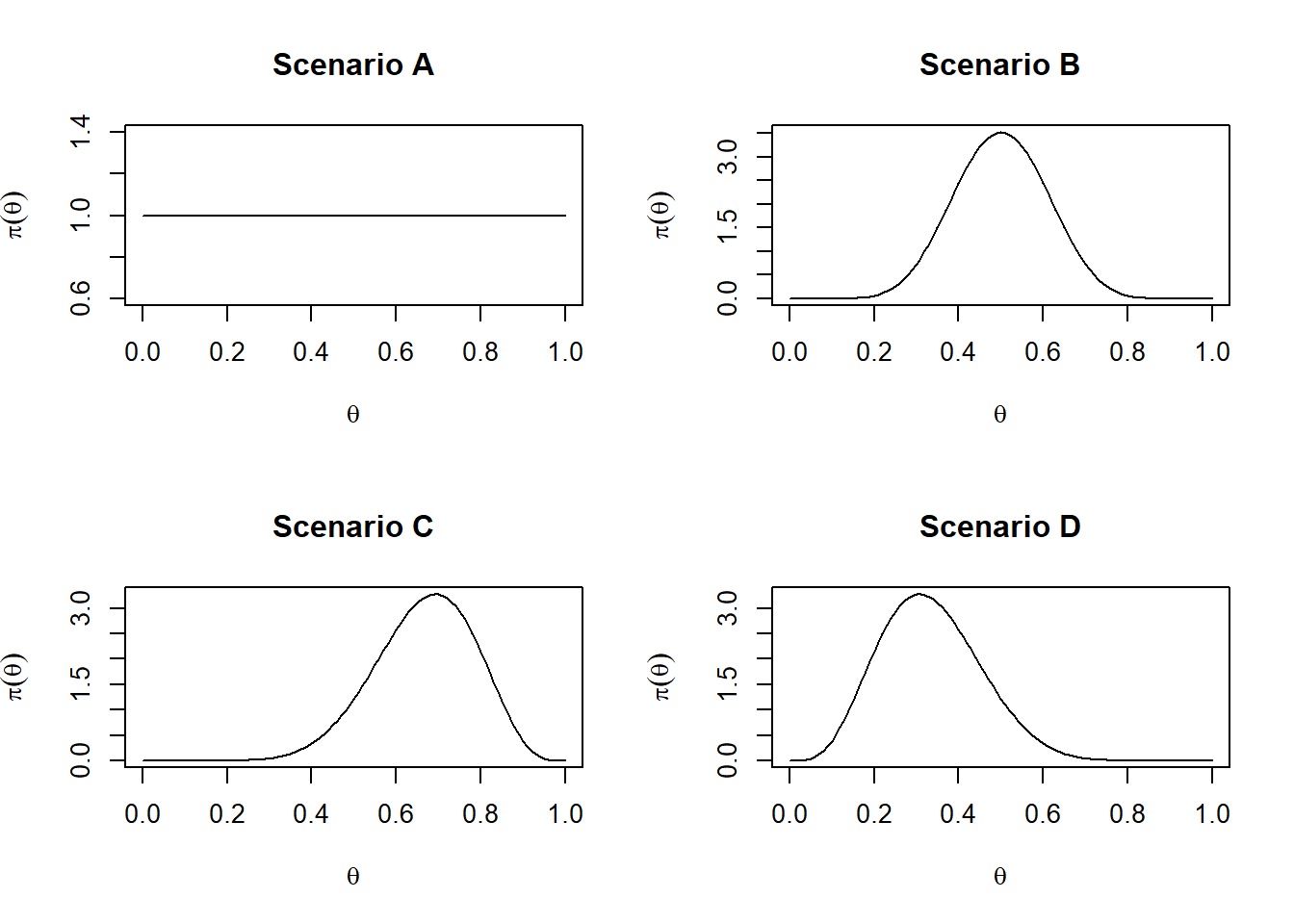
We will examine four different scenarios, each corresponding to a distinct choice of hyperparameters for the Beta prior.
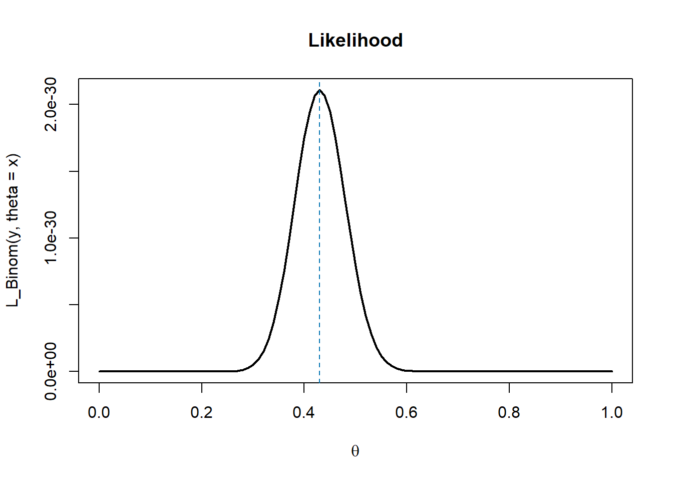
We further define the L_binom function, which returns the value of the likelihood function evaluated in a specific theta point.
L_Binom <-function(y, theta){ s <-sum(y) n <-length(y) L <- theta^s * (1-theta)^(n-s)return(L)}L_Binom(y, theta=0.001)
[1] 9.445671e-130
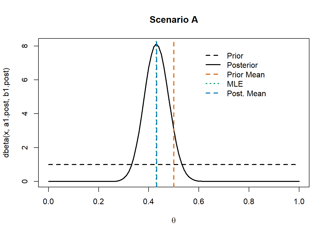
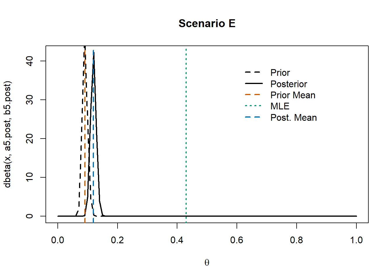
Obviously, the likelihood function does not depend on the prior distribution we impose on \(\theta\). In this case, the MLE corresponds to the sample mean (blue dashed line).
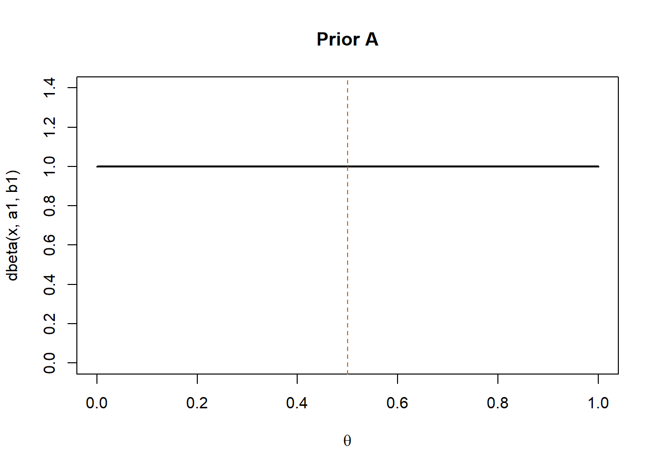
In this scenario, the prior distribution coincides with a uniform distribution on the \((0,1)\) interval. Thus, the prior mean (red dashed line) is equal to 0.5.
The chosen prior distribution does not favor any particular value of \(\theta\). Thus, we selected a non-informative prior. As a result, the posterior distribution is centered around the maximum likelihood estimate (MLE).
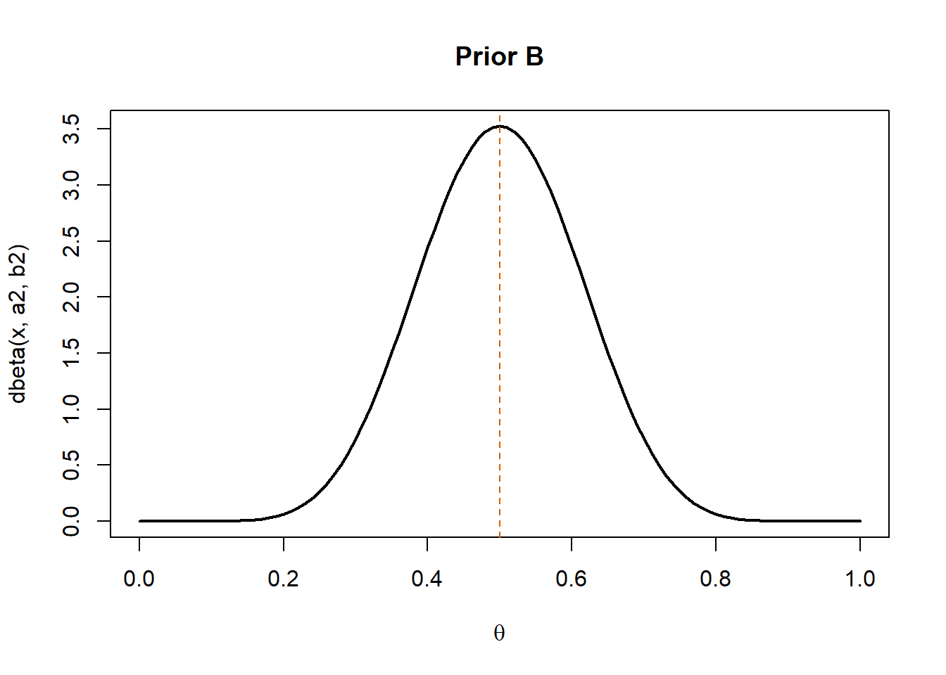
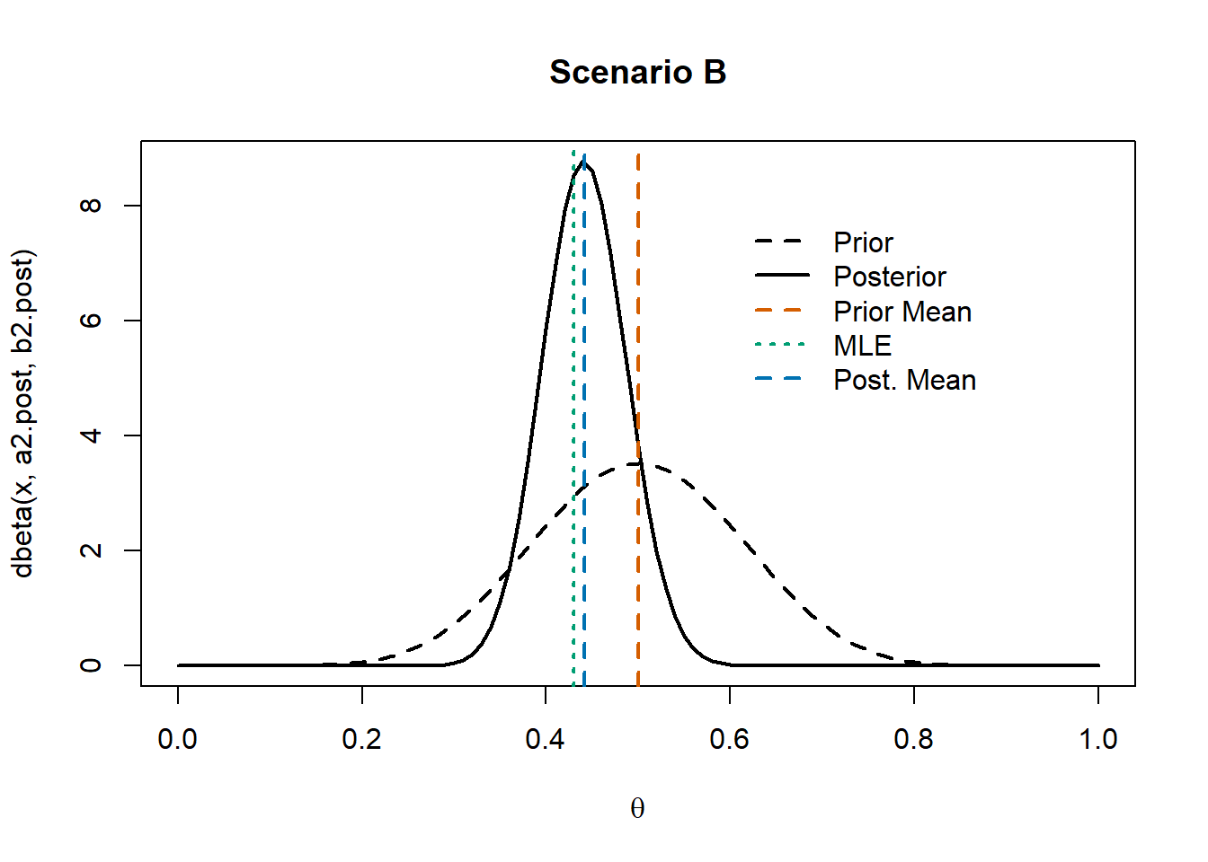
Scenario B
In this scenario, we use a prior distribution for \(\theta\) that is still symmetric (meaning it treats values below and above 0.5 in the same way). However, unlike the uniform prior, it is not flat: it expresses a preference for values closer to 0.5.
Since we are still considering a symmetric prior, the prior mean is equal to 0.5. However, unlike the uniform prior, it does not assign the same probability density to every value or interval of \(\theta\). As a consequence, the posterior mean becomes a weighted average between the prior mean and the MLE.
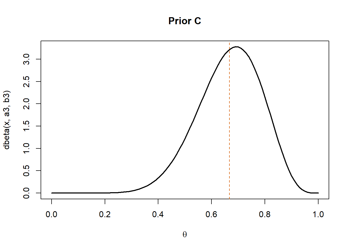
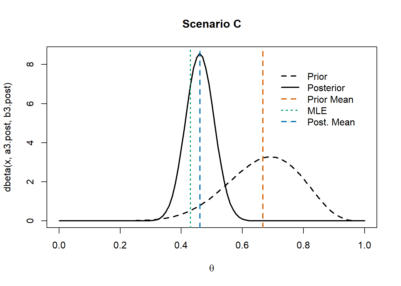
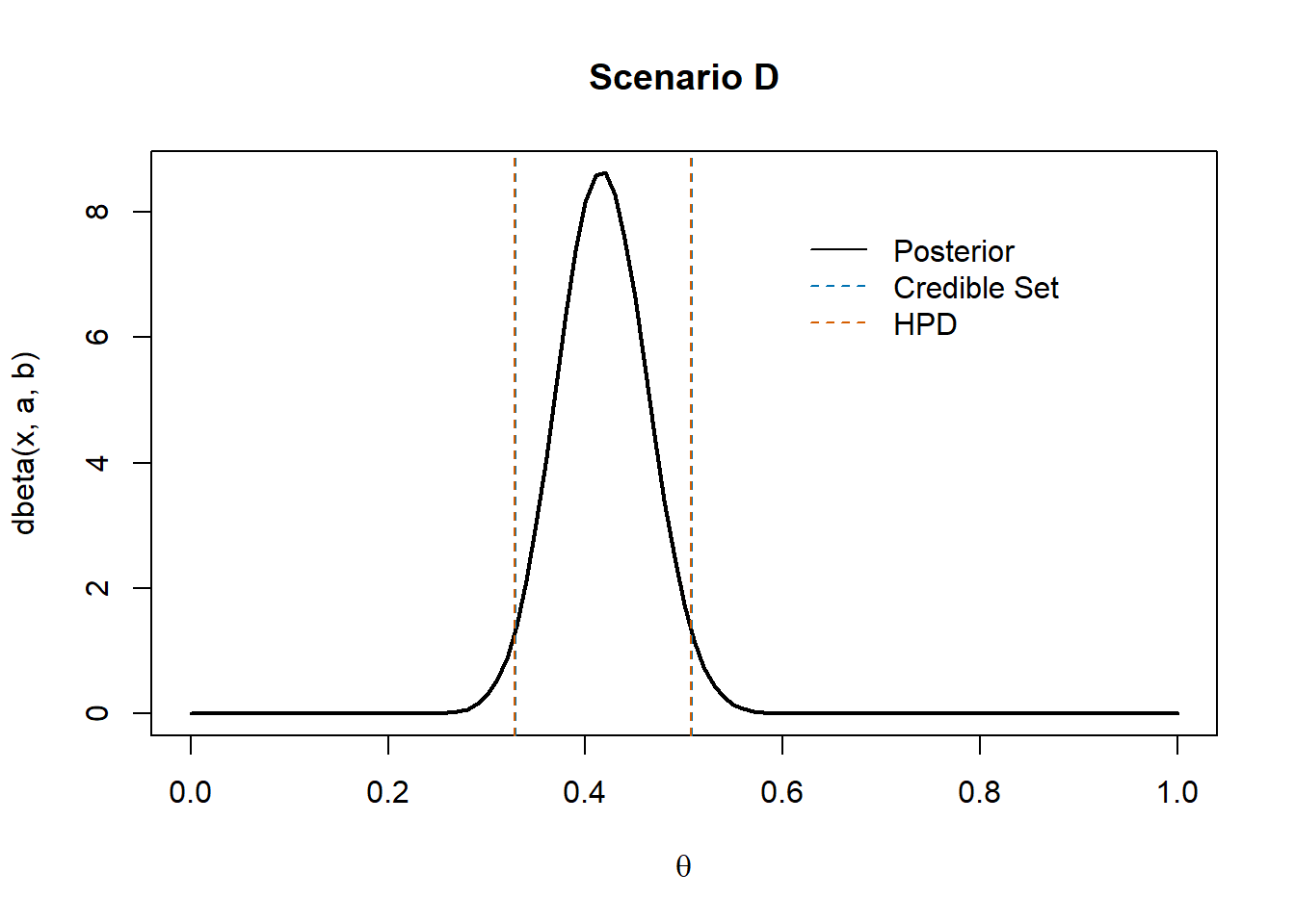
Scenario C & D
Scenarios C and D consider asymmetric prior distributions.
We may summarize the (prior and) posterior distribution by some measures:
Beta.Exp <-function(a, b) a/(a+b)Beta.Var <-function(a, b)(a*b)/((a+b)^2*(a+b+1))Beta.Mode <-function(a, b){ifelse(a>1& b>1, (a-1)/(a+b-2), NA)}Beta.Median <-function(a, b) qbeta(.5, a, b)
measures <-matrix(NA, ncol =6, nrow =4)rownames(measures) <-c("A", "B", "C", "D")colnames(measures) <-c("a.post", "b.post", "Exp", "Mode", "Median", "Var")measures[,1] <-c(a1.post, a2.post, a3.post, a4.post)measures[,2] <-c(b1.post, b2.post, b3.post, b4.post)for(i in1:4){ a <- measures[i,1] b <- measures[i,2] measures[i,3] <-Beta.Exp(a, b) measures[i,4] <-Beta.Mode(a, b) measures[i,5] <-Beta.Median(a, b) measures[i,6] <-Beta.Var(a, b)}round(measures,4)
  a.post b.post    Exp   Mode Median    Var
A     44     58 0.4314 0.4300 0.4309 0.0024
B     53     67 0.4417 0.4407 0.4413 0.0020
C     53     62 0.4609 0.4602 0.4606 0.0021
D     48     67 0.4174 0.4159 0.4169 0.0021
In this simple setting, even when using different priors, the resulting posterior distributions do not lead to substantially different point estimates. This happens because the empirical evidence (i.e., the information provided by the sample y) is much stronger than the prior beliefs.
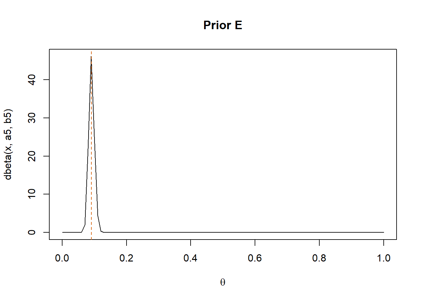
To better illustrate the impact of a strong prior, we now consider an additional scenario where we strongly believe that most people do not have cardiovascular disease.
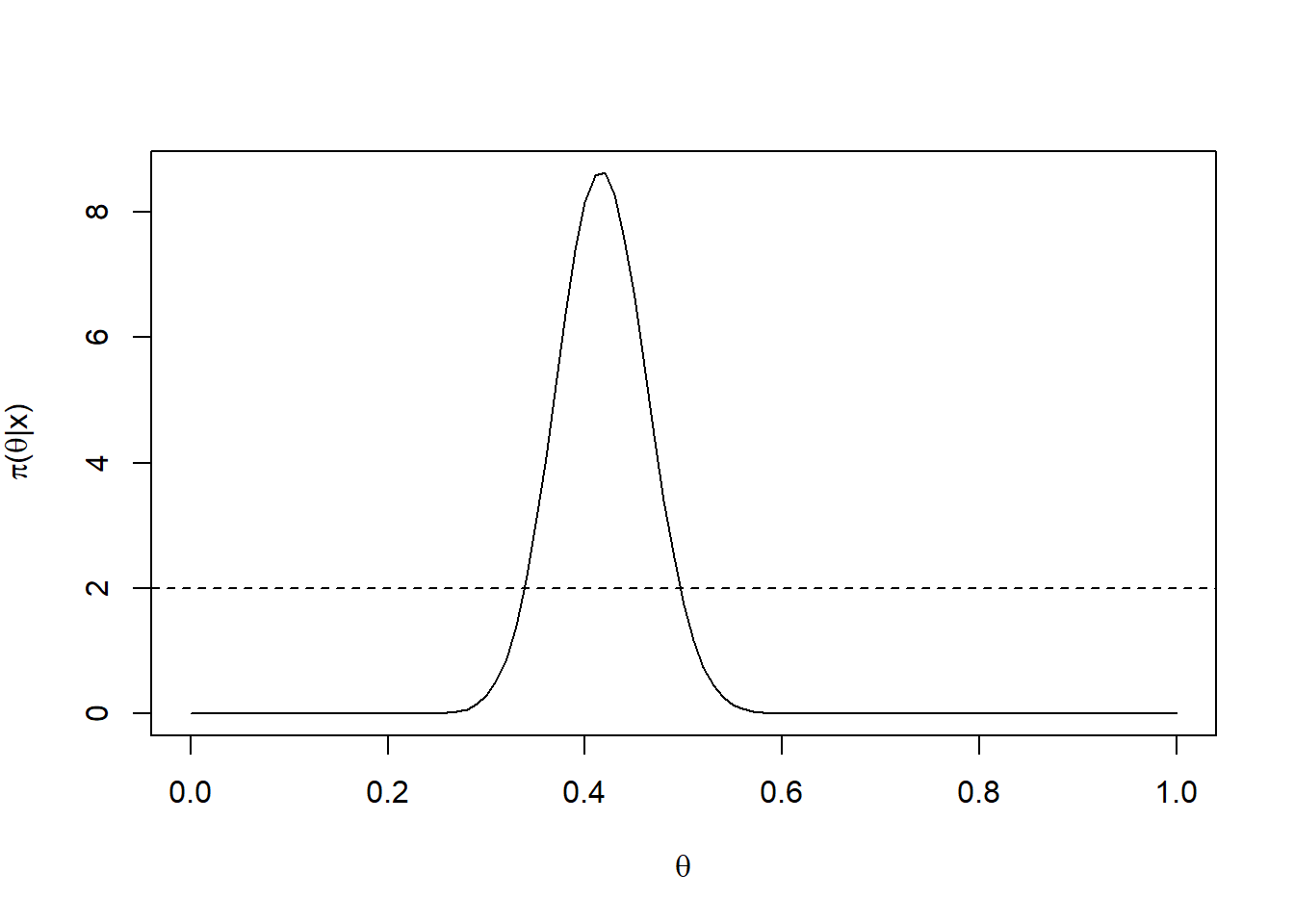
Let’s start by considering an initial value for \(h\).
h <-2curve(dbeta(x, a, b), ylab=expression(paste(pi,"(",theta,"|x)")),xlab=expression(theta))abline(h=h,lty=2)
We need to find the values of theta such that \(P(\theta|\textbf{y}) = h\).
To do this, we progressively lower the posterior density curve by an amount \(h\).
curve(dbeta(x, a, b), ylab=expression(paste(pi,"(",theta,"|x)")),xlab=expression(theta))abline(h=h,lty=2)translated <-function(x, a, b) dbeta(x,a, b) - h curve(translated(x, a, b), add = T, lty =3, lwd =2)abline(h =0, lty =3)
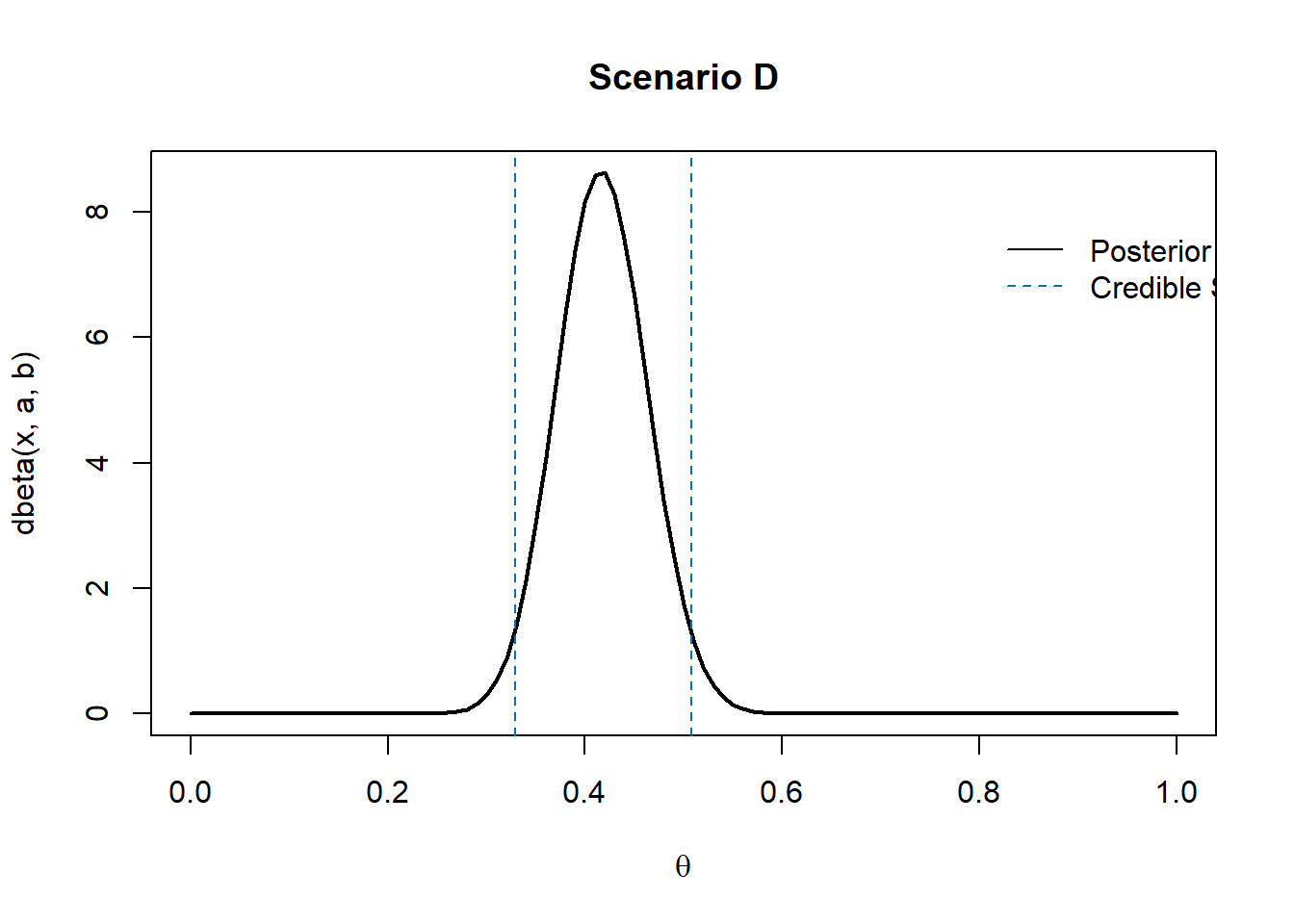
The values we are looking for are those where the translated curve —that is, the original posterior density minus \(h\)— becomes zero.
We have a probability equal to 0.9152. Thus, we have to select a smaller \(h\). Iteratively:
h.grid <-seq(1, 2, by =0.01) res <-matrix(NA, ncol=4, nrow=length(h.grid))colnames(res) <-c("HPD1", "HPD2", "level", "h")for(i in1:length(h.grid)){ translated <-function(x, a, b) dbeta(x,a, b) - h.grid[i] hpd1<-uniroot(translated,c(.2,.4),a,b)$root hpd2<-uniroot(translated,c(.43,.55),a,b)$root I <-integrate(dbeta, lower=hpd1, upper=hpd2, shape1=a, shape2=b)$value iter <- i res[i,] <-c(hpd1, hpd2, I, h.grid[i])if(I <=0.95) break}res[1:iter,]
Data do not support \(H_0\): by adding data to the prior belief, our confidence on \(H_0\) strongly decreases
HOMEWORK
Consider a sample of size \(n = 10\) composed of Bernoulli trials, for which we observed \(s = 3\) successes. Consider the prior \(\theta \sim Beta(2, 8)\).
Compute the posterior distribution of theta.
Compute the MLE and the prior and posterior means.
Compute and compare the 95% CS and HPD.
Let \(H_0 : \theta \in (0.3, 0.5)\) vs. \(H_1 : \theta \in (0, 0.3) \cup (0.5, 1)\). Which hypothesis do you support?