Script 2 - Normal & Monte Carlo Approximations

Author

Roberto Ascari

Normal Approximation for the Bernoulli-Beta posterior:

Let us consider results of a general election, where party A collected 150’000 votes out of the 240’000 total votes.

sum_y <- 150000
n <- 240000

We still consider the Bernoulli-Beta model, meaning that \(Y_i | \theta \sim Bernoulli(\theta)\) and \(\theta \sim Beta(a, b)\). Thus, \[\theta | \textbf{y} \sim Beta\left(a + \sum_{i=1}^n y_i, b + n - \sum_{i=1}^n y_i\right).\]

As for the choice of the hyperparameters \(a\) and \(b\), we consider results of a previous general election. In that election, party A collected 49’000 votes out of 270’000 total votes:

a <- 49000
b <- 270000

The Normal approximation requires the evaluation of the posterior mode. Let’s definte the mode of a Beta distribution.

Beta.Mode <- function(a, b){
  ifelse(a>1 & b>1, (a-1)/(a+b-2), NA)
}

The updated hyperparameters and the posterior mode \(\tilde{\theta}\) are:

a.post <- a + sum_y; a.post

[1] 199000

b.post <- b + n - sum_y; b.post

[1] 360000

post.mode <- Beta.Mode(a.post, b.post); post.mode

[1] 0.3559923

Finally, the variance of the approximated normal distribution, namely the inverse of \[\left. -\frac{\partial^2 \log \pi(\theta | \textbf{y})}{\partial \theta^2} \right|_{\theta = \tilde{\theta}}.\]

sigma_approx <- ((a.post-1)/(post.mode^2) + (b.post-1)/(1-post.mode)^2)^(-1)

sigma_approx

[1] 4.101299e-07

Let’s compare the true posterior distribution with its Normal approximation:

curve(dbeta(x, a.post, b.post), xlim=c(.35,.36), lty = "dashed")
curve(dnorm(x, post.mode, sqrt(sigma_approx)), add=T, col="#D55E00", lty = "dotted")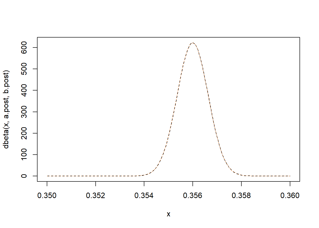

The Normal approximation is quite useful in computing HPDs, since they coincide with CSs due to the simmetry of the Normal distribution.

Iterative way for computing the true HPD:

h.grid <- seq(100, 105, by = 0.001)

res <- matrix(NA, ncol=4, nrow=length(h.grid))
colnames(res) <- c("HPD1", "HPD2", "level", "h")

for(i in 1:length(h.grid)){
  translated <- function(x, a, b) dbeta(x,a, b)-h.grid[i]

  hpd1<-uniroot(translated,c(.34,post.mode-.0005),a.post,b.post)$root
  hpd2<-uniroot(translated,c(post.mode+.0005,.36),a.post,b.post)$root

  I <- integrate(dbeta, lower=hpd1, upper=hpd2, shape1=a.post, shape2=b.post)$value

  iter <- i
  res[i,] <- c(hpd1, hpd2, I, h.grid[i])
  if(I <= 0.95) break
}

res[iter,]

       HPD1        HPD2       level           h 
  0.3547393   0.3572496   0.9499997 102.0680000

HPD <- res[iter-1,-c(3,4)]; HPD

     HPD1      HPD2 
0.3547393 0.3572496

HPD by taking advantage of the Normal approximation:

qnorm(c(.025,.975), post.mode, sqrt(sigma_approx))

[1] 0.3547371 0.3572475

Monte Carlo

When it is not possible to compute some quantity of interest directly from the posterior distribution, but it is possible to generate (pseudo)random samples from it, we can use Monte Carlo (MC) approximation methods.

Let us consider the following example.

A biostatistician aims to compare two treatments: - 1) a new vaccine for COVID-19; - 2) a placebo.

He/She collects a sample of 200 patients and randomly assigns them into two groups of equal size.

n1 <- 100
n2 <- 100

The first group receives the new vaccine, while the second group receives the placebo.

After the treatments, the biostatistician records the number of deaths in each group, denoted by \(Y_1\) and \(Y_2\), respectively.

\(Y_1|\theta_1 \sim Bernoulli(\theta_1)\)

\(Y_2| \theta_2 \sim Bernoulli(\theta_2)\)

\(\theta_j\) represents the probability of death in group \(j\).

The biostatistician chooses to use non-informative priors for the parameters.

a1 <- 1
b1 <- 1

a2 <- 1
b2 <- 1

Once the priors have been selected, he/she looks at the data…

s1 <- 20
s2 <- 80

… and updates the prior hyperparameters to obtain the posterior distributions.

a1.post <- a1 + s1
b1.post <- b1 + n1 - s1

a2.post <- a2 + s2
b2.post <- b2 + n2 - s2

curve(dbeta(x ,a1.post,b1.post), 0,1, lty=1, ylim=c(0,10),
      xlab=expression(theta), ylab=expression(pi), lwd=2)
curve(dbeta(x , a2.post, b2.post), add=T, lty=3, lwd=2)
legend(0.4,10,c("Posterior 1","Posterior 2"),lty=c(1,3),cex=0.8,lwd=2,bty="n")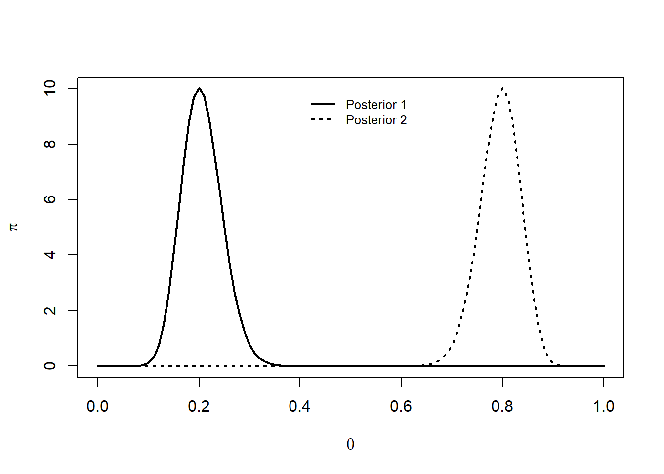

These posterior distributions suggest that \(\theta_1\) and \(\theta_2\) are concentrated around different values.

The biostatistician’s goal is to study the log odds ratio \[\eta = \log \frac{\frac{\theta_1}{1-\theta_1}}{\frac{\theta_2}{1-\theta_2}}.\] It is important to note that while we have obtained the posterior distributions of \(\theta_1\) and \(\theta_2\), we have not directly computed the posterior distribution of \(\eta\).

B <- 100000

set.seed(42)
theta1 <- rbeta(B, a1.post, b1.post)
theta2 <- rbeta(B, a2.post, b2.post)

eta <- log(theta1/(1-theta1)*(1-theta2)/theta2)

# Posterior Mean:
mean(eta)

[1] -2.735187

# Posterior Variance:
var(eta)

[1] 0.1222466

# CS
CS <- quantile(eta, p=c(.025,.975)); CS

     2.5%     97.5% 
-3.433526 -2.066745

# Histogram and kernel estimate:

hist(eta, prob=T, xlab=expression(eta), main="Posterior distribution of log OR")
lines(density(eta), col="#D55E00")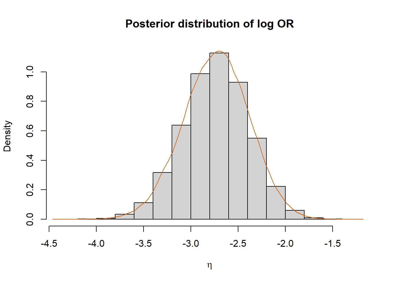

Using Monte Carlo sampling, the biostatistician estimates that, with 95% probability, the log odds ratio falls within the interval (-3.433526, -2.0667447).
This indicates that the odds of death in the “Vaccine” group are significantly lower than those in the “Placebo” group.