You can download the R script here .
Some useful links for working with Stan:
Linear Regression
In this part, we are going to fit a simple linear regression model through Stan. Here you can download the .stan model.
First of all, let’s compile the model and save it into an R object.
<- rstan:: stan_model (file= "data/LM_Model.stan" )
S4 class stanmodel 'anon_model' coded as follows:
data{
    int<lower = 0> n;  // number of obs
    int<lower = 0> K;  // number of covariates (including the intercept)

    vector[n] y;     // response
    matrix[n, K] X;  // covariates
  real a0;
  real b0;
    vector[K] beta0;
    vector[K] s2_0;
}
parameters{
    real<lower = 0> sigma2;
    vector[K] beta;
}
transformed parameters {
    vector[n] mu;
  mu = X * beta;
}
model{
    // Prior:
    sigma2 ~ inv_gamma(a0, b0);

    for(k in 1:K){
        beta[k] ~ normal(beta0[k], sqrt(s2_0[k]));
    }
    // Likelihood:
    y ~ normal(mu, sqrt(sigma2));
}
generated quantities{

    vector[n] log_lik;

    for (j in 1:n){
            log_lik[j] = normal_lpdf(y[j] | mu[j], sqrt(sigma2));
    }
}
We consider the Prestige data from the car package. Statistical units are occupations, for which we have:
education: average education of occupational incumbents, years, in 1971;
income: average income of incumbents, dollars, in 1971;
women: percentage of incumbents who are women;
prestige: Pineo-Porter prestige score for occupation, from a social survey conducted in the mid-1960s;
census: canadian Census occupational code;
type: type of occupation (bc, Blue Collar; prof, Professional, Managerial, and Technical; wc, White Collar).
Let’s transform the income variable so to reduce the asimmetry.
data ("Prestige" )<- complete.cases (Prestige),- 5 ]$ income <- log (Prestige2$ income)
In order to fit the stan model, we need to pass some data: - y: the response vector;
X: the design matrix;
n: the sample size;
K: the number of covariates (including the intercept term);
a0, b0, beta0, s2_0: hyperparameters.
<- Prestige2$ prestige<- lm (prestige ~ ., data= Prestige2)<- model.matrix (mod)<- nrow (X)<- ncol (X)
We further create a list containing the objects to be passed to the stan model.
<- list (y = y,X = X,n = n,K = K,a0 = 10 ,b0 = 10 ,beta0 = rep (0 , K),s2_0 = rep (10 , K)
We can now use the rstan::sampling function to fit the model. We want two chains, each of length 10’000, and we want to discard the first 50% as warm-up.
<- 10000 <- 2 <- rstan:: sampling (object = LM_Model,data = data.stan,warmup = 0.5 * n.iter, iter = n.iter,thin= 1 , chains = nchain,refresh = n.iter/ 2 #, pars=c("beta", "sigma2")
SAMPLING FOR MODEL 'anon_model' NOW (CHAIN 1).
Chain 1:
Chain 1: Gradient evaluation took 0.000129 seconds
Chain 1: 1000 transitions using 10 leapfrog steps per transition would take 1.29 seconds.
Chain 1: Adjust your expectations accordingly!
Chain 1:
Chain 1:
Chain 1: Iteration:    1 / 10000 [  0%]  (Warmup)
Chain 1: Iteration: 5000 / 10000 [ 50%]  (Warmup)
Chain 1: Iteration: 5001 / 10000 [ 50%]  (Sampling)
Chain 1: Iteration: 10000 / 10000 [100%]  (Sampling)
Chain 1:
Chain 1:  Elapsed Time: 1.32 seconds (Warm-up)
Chain 1:                1.611 seconds (Sampling)
Chain 1:                2.931 seconds (Total)
Chain 1:

SAMPLING FOR MODEL 'anon_model' NOW (CHAIN 2).
Chain 2:
Chain 2: Gradient evaluation took 1.1e-05 seconds
Chain 2: 1000 transitions using 10 leapfrog steps per transition would take 0.11 seconds.
Chain 2: Adjust your expectations accordingly!
Chain 2:
Chain 2:
Chain 2: Iteration:    1 / 10000 [  0%]  (Warmup)
Chain 2: Iteration: 5000 / 10000 [ 50%]  (Warmup)
Chain 2: Iteration: 5001 / 10000 [ 50%]  (Sampling)
Chain 2: Iteration: 10000 / 10000 [100%]  (Sampling)
Chain 2:
Chain 2:  Elapsed Time: 1.369 seconds (Warm-up)
Chain 2:                1.536 seconds (Sampling)
Chain 2:                2.905 seconds (Total)
Chain 2:
<- summary (LM_stan, pars = c ("beta" , "sigma2" ))$ summaryrownames (summ)[1 : K] <- colnames (X)round (summ, 3 )
              mean se_mean    sd   2.5%    25%    50%    75%  97.5%    n_eff
(Intercept) -3.012   0.040 3.079 -9.140 -5.104 -2.977 -0.930  2.954 6033.655
education    4.304   0.007 0.456  3.400  3.999  4.298  4.599  5.213 3981.793
income       0.516   0.010 0.607 -0.679  0.113  0.527  0.910  1.718 4052.160
women       -0.060   0.000 0.025 -0.109 -0.076 -0.060 -0.043 -0.013 6493.318
typeprof     6.086   0.034 2.306  1.545  4.540  6.108  7.632 10.607 4573.710
typewc      -2.792   0.023 1.798 -6.258 -3.997 -2.794 -1.600  0.819 6341.193
sigma2      48.760   0.083 6.631 37.422 44.093 48.226 52.723 63.571 6315.024
             Rhat
(Intercept) 1.000
education   1.000
income      1.000
women       1.000
typeprof    1.000
typewc      1.000
sigma2      1.001
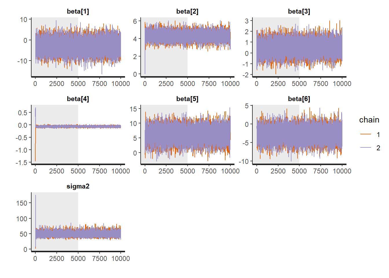
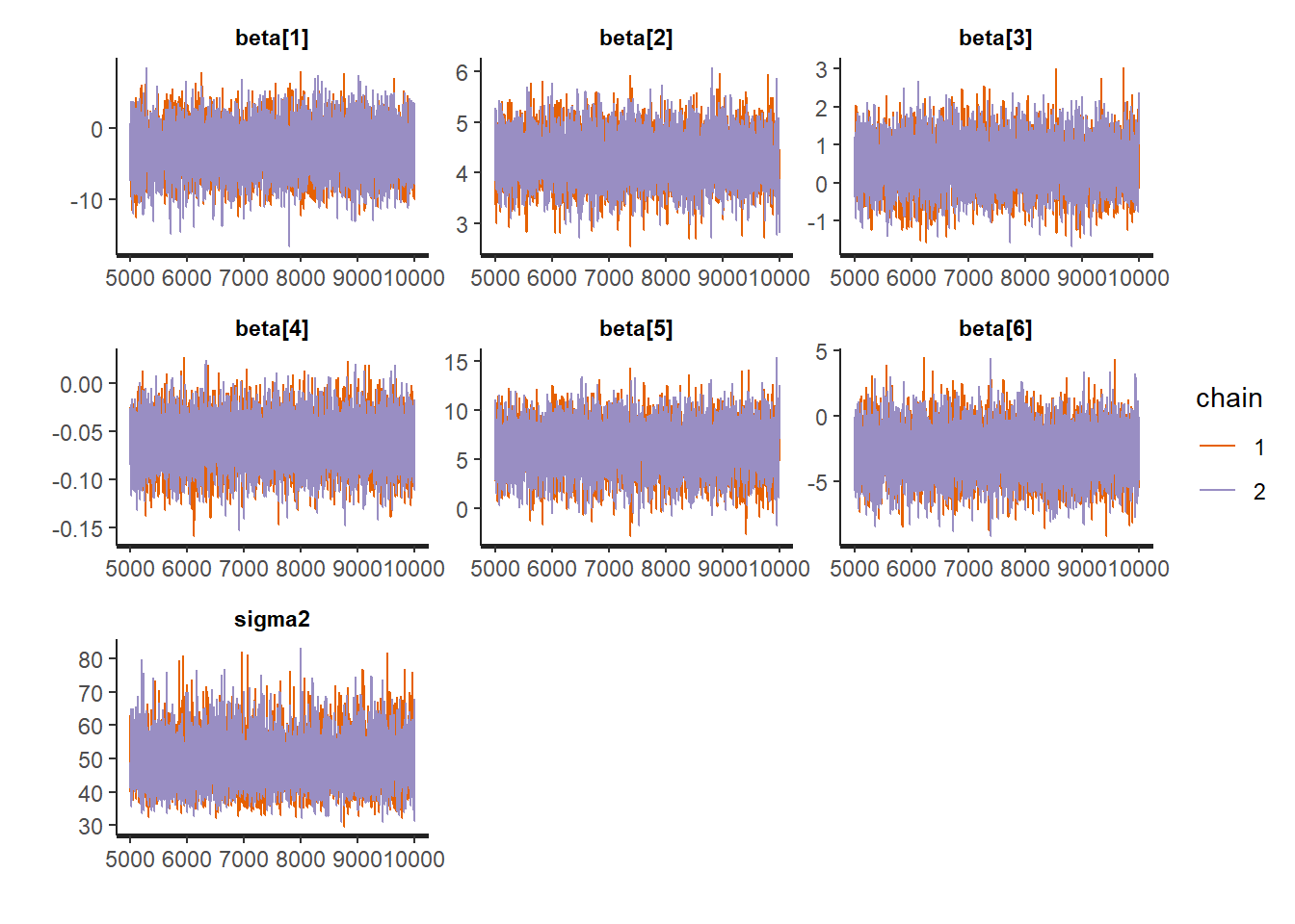
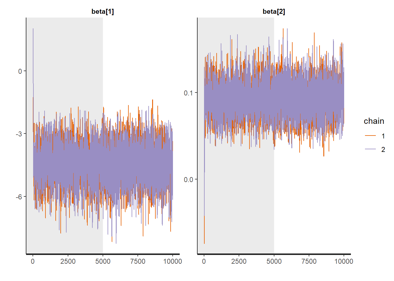
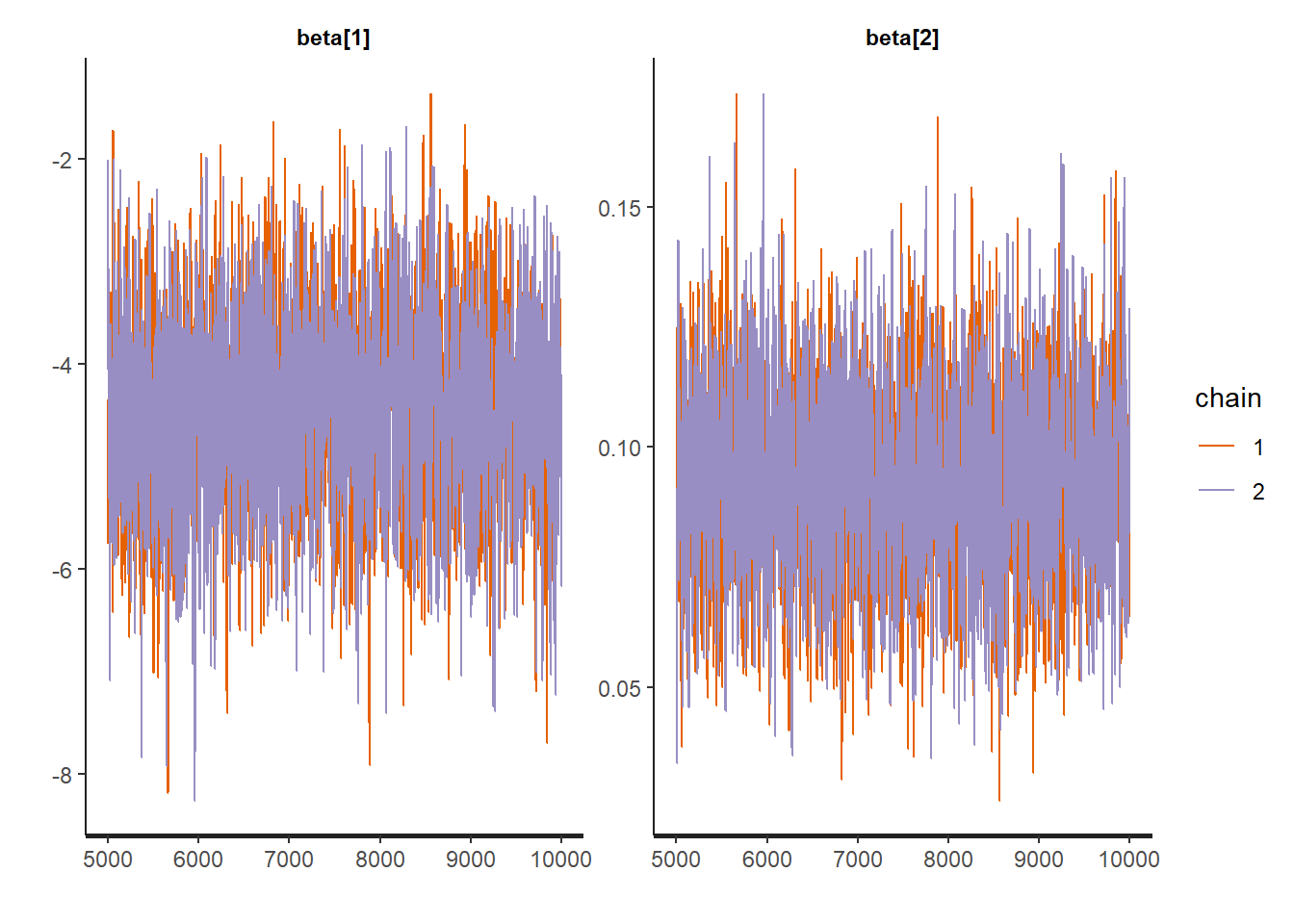
Traceplots:
:: traceplot (LM_stan, pars = c ('beta' , 'sigma2' ), inc_warmup = TRUE ):: traceplot (LM_stan, pars = c ('beta' , 'sigma2' ), inc_warmup = FALSE )
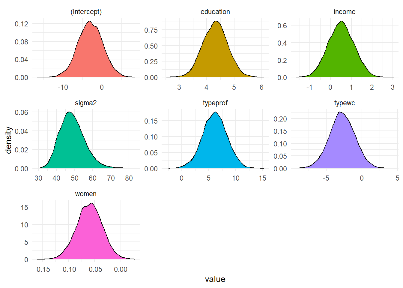
<- rstan:: extract (LM_stan, c ('beta' , 'sigma2' )) <- post_chain$ betacolnames (betas) <- colnames (X)<- post_chain$ sigma2<- data.frame (value = c (1 ], betas[,2 ], betas[,3 ],4 ], betas[,5 ], betas[,6 ],param = rep (c (colnames (X), 'sigma2' ), each = nrow (post_chain$ beta)))%>% ggplot (aes (value, fill = param)) + geom_density () + facet_wrap (~ param, scales = 'free' ) + theme_minimal () + theme (legend.position= "false" )
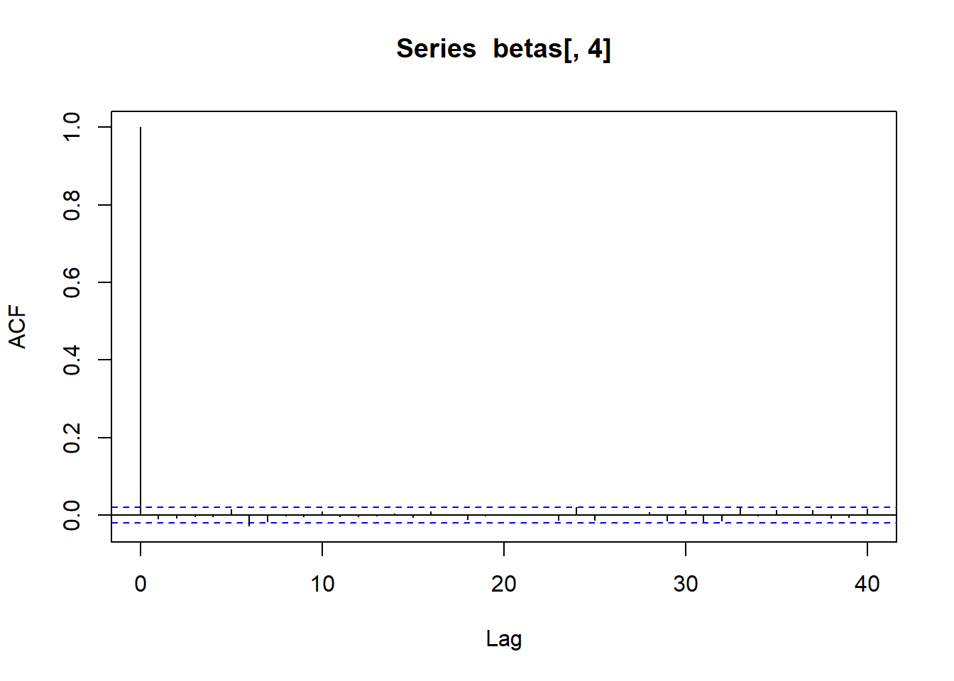
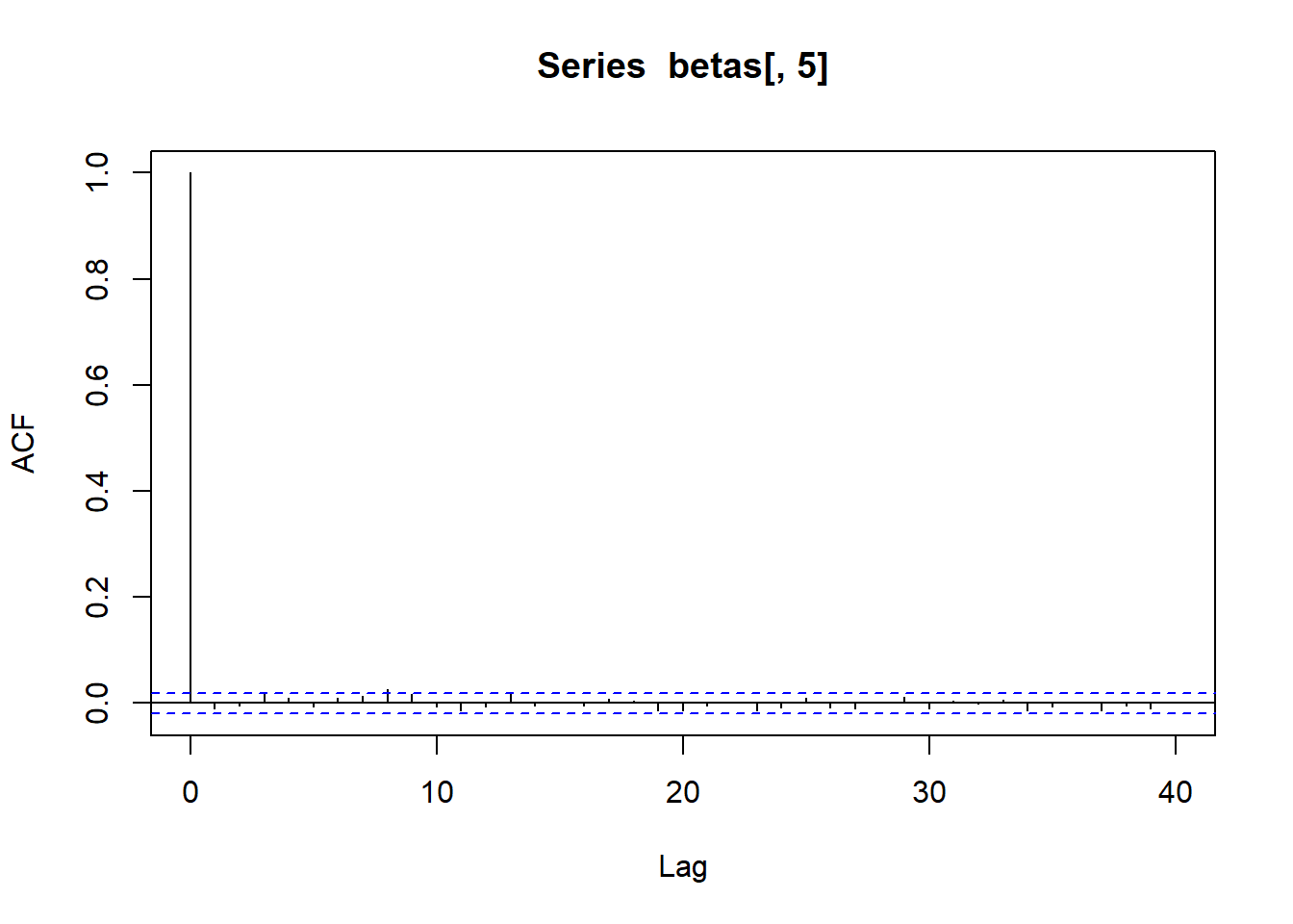
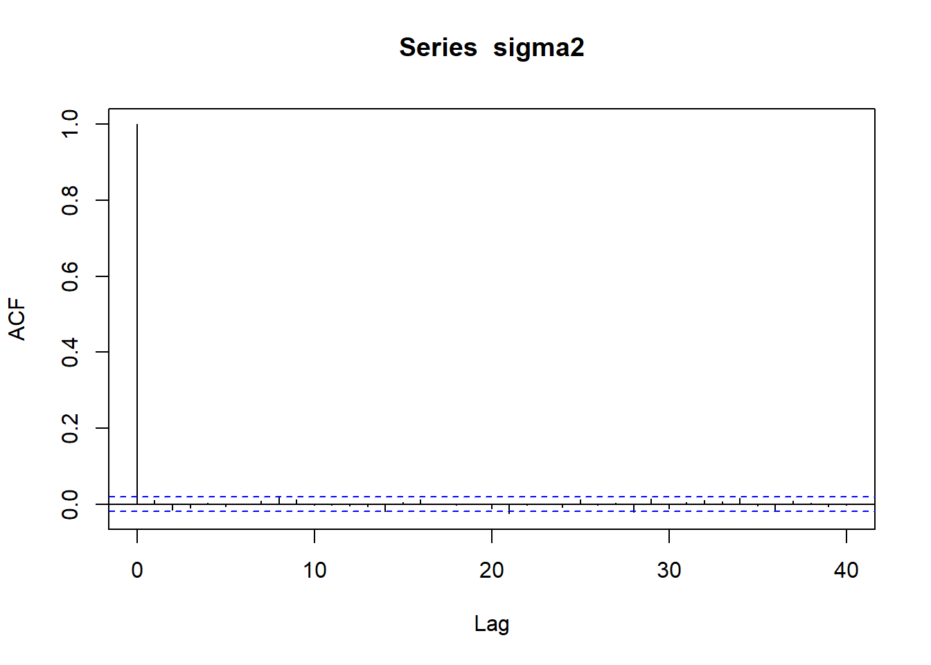
acf (betas[,5 ])acf (betas[,5 ])
As classical MCMCs, we can use the sampled values to approximate any quantity of interest. For example, we can approximate \(\mathbb{P}(\beta_1 > 4, \beta_3 > -0.5)\) :
mean (betas[,2 ] > 4 & betas[,4 ] > - .5 )
Logistic Regression
Let’s consider the logistic regression model to the cardiac dataset .
The Logistic_Model.stan model can be downloaded here .
rm (list = ls ())<- read.csv ("data/cardiac.csv" , header= T, sep= ";" )<- cardiac$ Chd<- model.matrix (lm (Chd ~ ., data= cardiac))<- nrow (X)<- ncol (X)
<- :: stan_model (file= "data/Logistic_Model.stan" )
S4 class stanmodel 'anon_model' coded as follows:
///////////////////////// DATA /////////////////////////////////////
data {
    int<lower = 1> n;       // number of data
    int<lower = 1> K;       // number of covariates (including the intercept)
    int<lower = 0, upper = 1> y[n];   // response vector
    matrix[n, K] X;           // design matrix

  vector[K] beta0;
  vector[K] s2_0;
}
//////////////////// PARAMETERS /////////////////////////////////
parameters {
    vector[K] beta;        // regression coefficients
}
transformed parameters {
    vector[n] eta;
    vector<lower=0>[n] Odds;
    vector<lower=0,upper=1>[n] p;

  eta = X * beta;

  for(i in 1:n){
    Odds[i] = exp(eta[i]);
    p[i] = Odds[i]/(1+Odds[i]);
  }

}
////////////////// MODEL ////////////////////////
model {
  // Prior
    for (j in 1:K){
        beta[j] ~ normal(beta0, sqrt(s2_0));
    }

  // Likelihood
    for (s in 1:n){
        y[s] ~ bernoulli(p[s]);
    }
}
<- list (y = y,X = X,n = n,K = K,beta0 = rep (0 , K),s2_0 = rep (10 , K)
<- 10000 <- 2 <- rstan:: sampling (object = Logistic_Model,data = data.stan_logis,warmup = 0.5 * n.iter, iter = n.iter,thin = 1 , chains = nchain,refresh = n.iter/ 2
SAMPLING FOR MODEL 'anon_model' NOW (CHAIN 1).
Chain 1:
Chain 1: Gradient evaluation took 7.5e-05 seconds
Chain 1: 1000 transitions using 10 leapfrog steps per transition would take 0.75 seconds.
Chain 1: Adjust your expectations accordingly!
Chain 1:
Chain 1:
Chain 1: Iteration:    1 / 10000 [  0%]  (Warmup)
Chain 1: Iteration: 5000 / 10000 [ 50%]  (Warmup)
Chain 1: Iteration: 5001 / 10000 [ 50%]  (Sampling)
Chain 1: Iteration: 10000 / 10000 [100%]  (Sampling)
Chain 1:
Chain 1:  Elapsed Time: 2.089 seconds (Warm-up)
Chain 1:                1.682 seconds (Sampling)
Chain 1:                3.771 seconds (Total)
Chain 1:

SAMPLING FOR MODEL 'anon_model' NOW (CHAIN 2).
Chain 2:
Chain 2: Gradient evaluation took 2.5e-05 seconds
Chain 2: 1000 transitions using 10 leapfrog steps per transition would take 0.25 seconds.
Chain 2: Adjust your expectations accordingly!
Chain 2:
Chain 2:
Chain 2: Iteration:    1 / 10000 [  0%]  (Warmup)
Chain 2: Iteration: 5000 / 10000 [ 50%]  (Warmup)
Chain 2: Iteration: 5001 / 10000 [ 50%]  (Sampling)
Chain 2: Iteration: 10000 / 10000 [100%]  (Sampling)
Chain 2:
Chain 2:  Elapsed Time: 1.569 seconds (Warm-up)
Chain 2:                1.196 seconds (Sampling)
Chain 2:                2.765 seconds (Total)
Chain 2:
<- summary (Logistic_stan, pars = "beta" )$ summaryrownames (summ)[1 : K] <- colnames (X)round (summ, 3 )
mean se_mean sd 2.5% 25% 50% 75% 97.5% n_eff
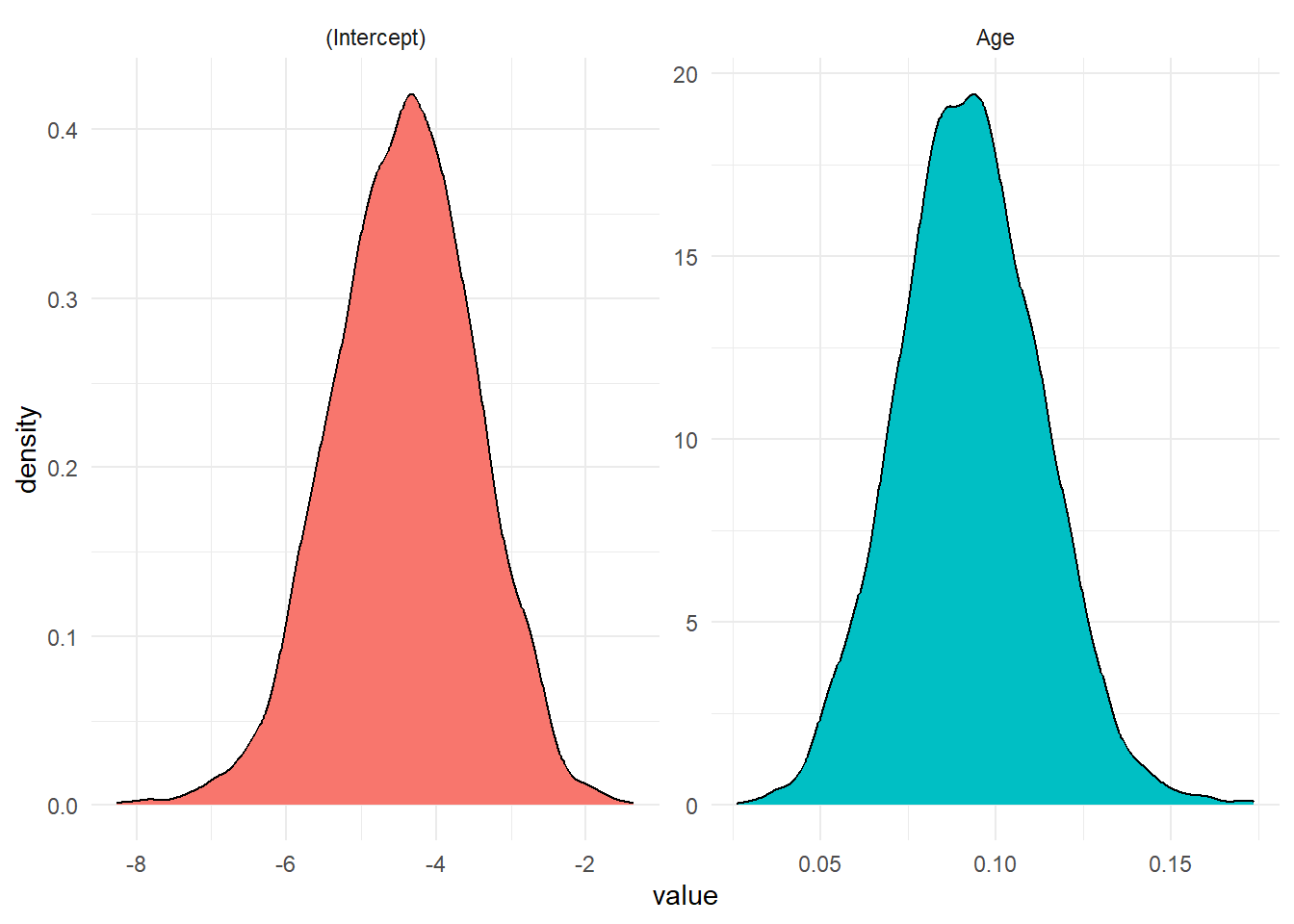
(Intercept) -4.417 0.023 0.963 -6.409 -5.051 -4.394 -3.737 -2.623 1773.845
Age 0.092 0.000 0.021 0.054 0.078 0.092 0.106 0.135 1783.732
Rhat
(Intercept) 1.002
Age 1.002
:: traceplot (Logistic_stan, pars = "beta" , inc_warmup = TRUE ):: traceplot (Logistic_stan, pars = "beta" , inc_warmup = FALSE )
<- rstan:: extract (Logistic_stan, "beta" ) <- post_chain$ betacolnames (betas) <- colnames (X)<- data.frame (value = c (betas[,1 ], betas[,2 ]), param = rep (colnames (X), each = nrow (post_chain$ beta)))%>% ggplot (aes (value, fill = param)) + geom_density () + facet_wrap (~ param, scales = 'free' ) + theme_minimal () + theme (legend.position= "false" )
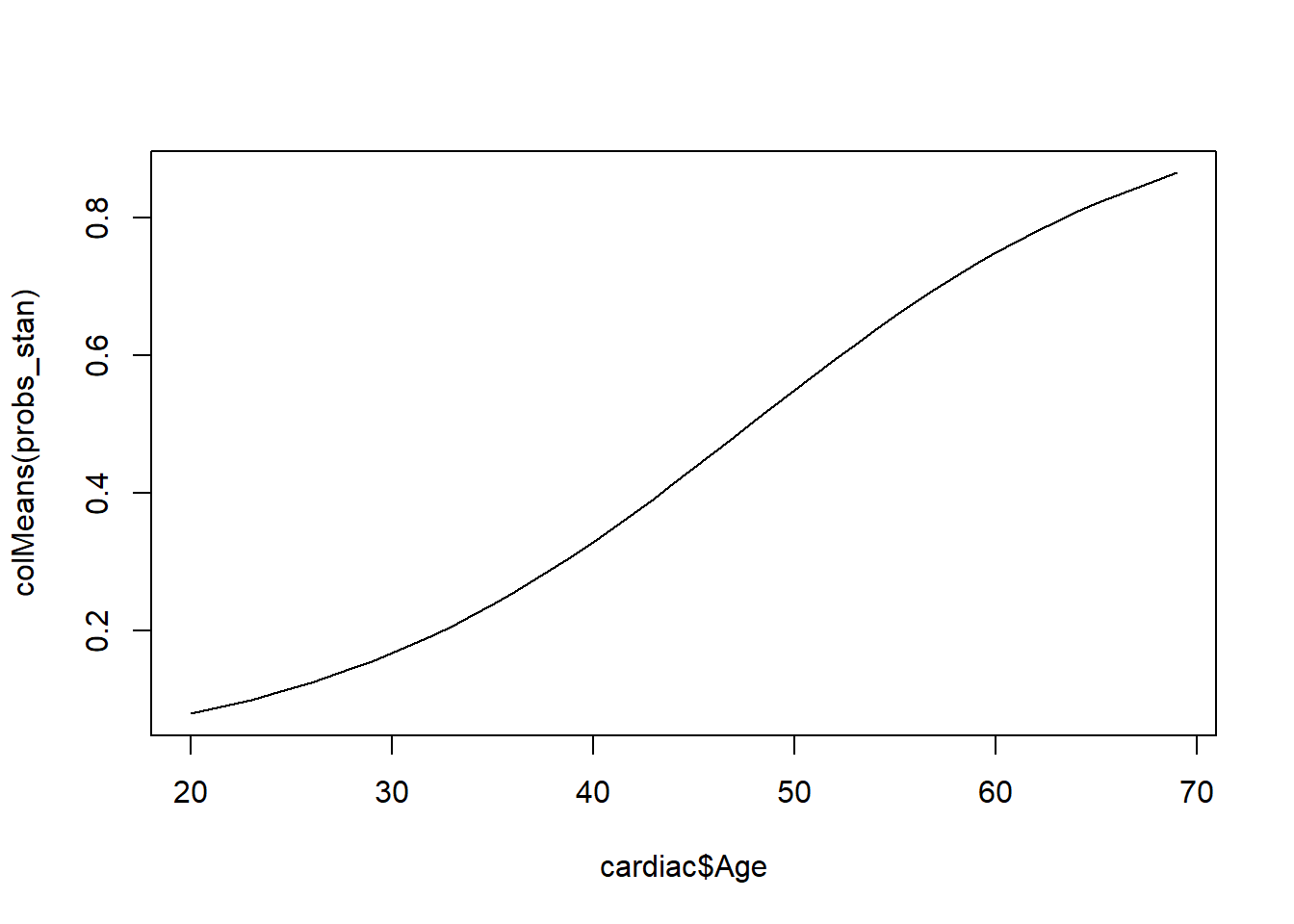
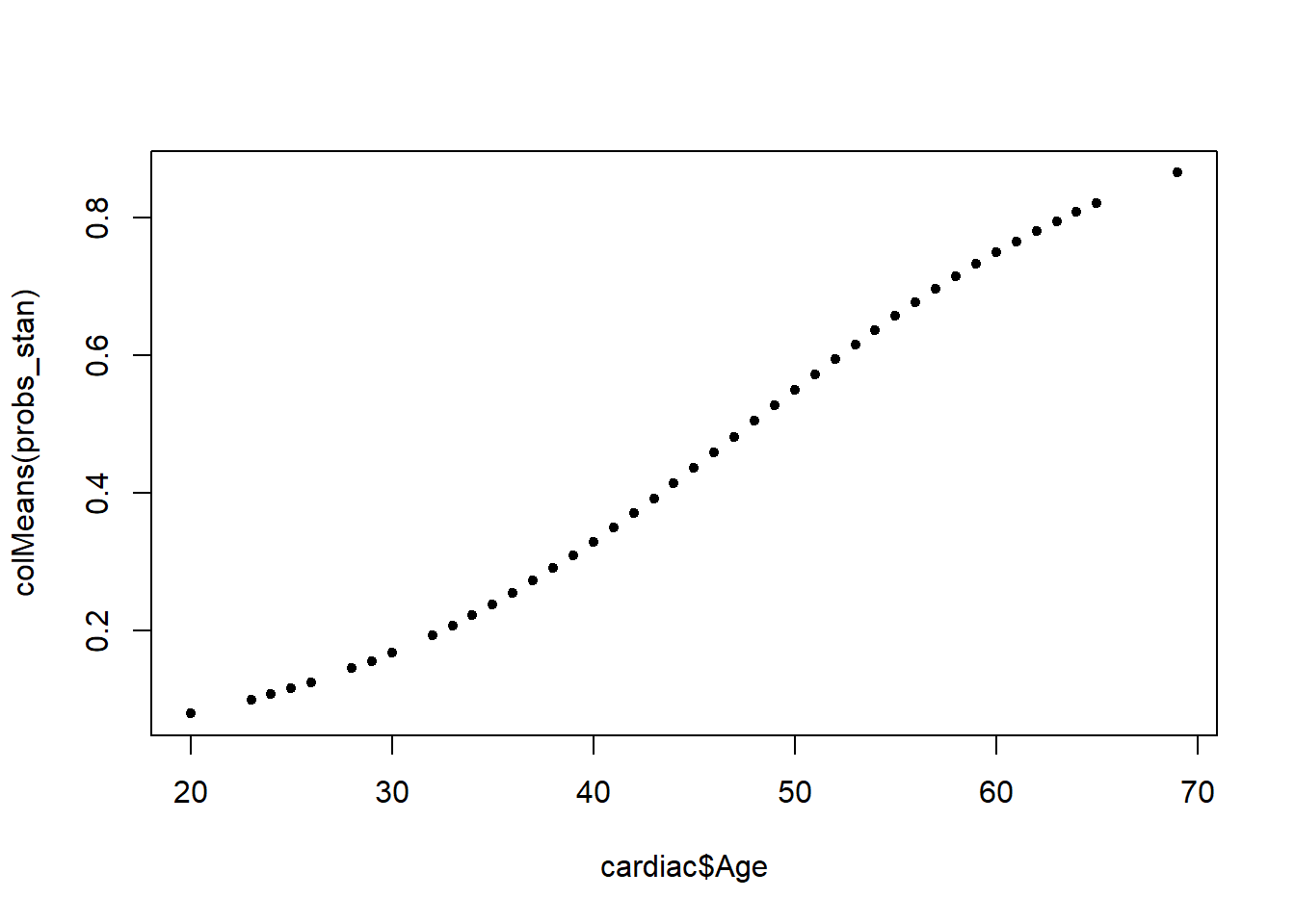
We can evaluate probabilities for each patients.
<- rstan:: extract (Logistic_stan, "p" )$ pplot (cardiac$ Age, colMeans (probs_stan), pch= 20 , type= "l" )plot (cardiac$ Age, colMeans (probs_stan), pch= 20 )